FILTER

The filter function is unique to Google Spread sheets, without this function extracting a duplicate records from a data table will be a very big arrayformula. The power of filter function is in its usage. we will try to understand the basic usage of this function.

The Syntax of Filter function is as follows
FILTER(sourceArray, arrayCondition_1, arrayCondition_2, …, arrayCondition_30)

Explanation given in the help file:

Returns a filtered version of the given source array, where only certain rows or columns have been included. Each condition should be either a 1-dimensional range of boolean values, or else an array-formula expression which evaluates to a 1-dimensional array of booleans. If the conditions evaluate to a column array, then only the rows from the source array corresponding to the true values of the condition array will be returned. Likewise, if the conditions evaluate to a row array, then only the columns of the source array corresponding to the true values in the condition will be returned. If there are multiple conditions, then all must be true for the corresponding values in the source array to be returned.

SourceArray:
The sourcearray is nothing but data source in which we want to apply certain conditions to extract the required results.

arraycondition_1, arrayCondition_2, …, arrayCondition_30 :
We can write the upto 30 conditions to filter the required results.

now lets try to understand the function with an example.

to filter the data we can do it in two ways

(1) Using filter icon  in the menu bar

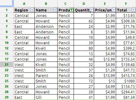
Adding a filter onto a set of data can help us quickly narrow down the data set to find the data we need. By selecting a data set, we can filter and sort amongst many rows at once. suppose if we want to filter the data table containing the value “Pencil”in the column C  

Step 1:
select the Filter icon in the menu bar as shown in the picture

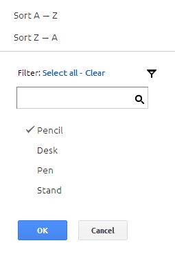
Step 2:
by selecting the pencil in the drop down menu as shown the picture below and press OK

The filtered data will be look like this:

The same results can be obtained using filter function in google docs spread sheet by using the following formula
=filter(A2:F30;C2:C30=”Pencil”)

Note: the formula should be entered in the after column F

we can further narrow down the results such as
if we want to filter the data where region is equal to West and Product is equal to Pencil the formula will be
=filter(A2:F30;A2:A30=”West”;C2:C30=”Pencil”)

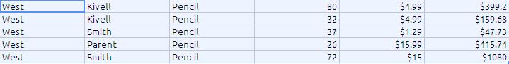
in the above formula the function is extracting the data using something like AND condition i.e. the data is shown as if the cell A2:A30 is West and cell C2:C30 is Pencil.

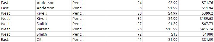
Similarly we can also evaluate the same formula for OR conditions. Suppose we want to extract data which full fills the following conditions:
Column A = West or East
Column C = Pencil

the formula will be
=filter(A2:F30;(A2:A30=”West”)+(A2:A30=”East”);C2:C30=”Pencil”) the results will be as shown below

The filter function can also be used for single condition or multiple conditional sum
=sum(filter(F2:F30;(A2:A30=”West”)+(A2:A30=”East”);C2:C30=”Pencil”))
it will give the sum of 71.76+11.94+399.2+159.68+47.73+415.74+1080+81.59 which is noting but total of last column of the above picture.

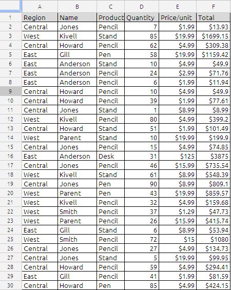
The data table used in this example: