Query function in Google Spreadsheets
November 1, 2013 28 Comments
Most versatile effective function and unique to Google Spreadsheets. I am documenting this function to understand it properly and for those who do not have programming background. I do not have previous experience with query. i will try to illustrate with examples.
If you have confusion and stuck some where please post your questions Google Docs forum at the following link https://productforums.google.com/forum/#!categories/docs/spreadsheets. There are experts in this area waiting for your questions.
Google Spreadsheet query is designed to be similar to SQL with few exceptions. it is a subset of SQL with a few feature of its own. if you are familiar with SQL it will be easy to learn.
The Syntax of the function is as follow:
QUERY(data, query, headers)
DATA: it can be columns(A:C open ranges) of data you want to query, range of cells such as A1:C10, result of function such as importrange, index etc.,
QUERY: It is similar to SQL with small exceptions there is no FROM clause in the this since DATA itself is acting like a FROM clause.
HEADERS: If your data has headers in the row you can specify this here (suppose your first row has headers you can specify this as 1)
Notes:
-
column headers have to capital letter such A, B, C if you are picking up the raw data with in the same spreadsheet.
-
if you are using the array formulas to manipulate the data (Index, Filter, importrange to name a few) then column headers will Col1, Col2, Col3 etc. observe i have used C capital letter in Col1. this is syntax you have to follow this otherwise you will get a parse error
-
parse error: an error of language resulting from code that does not conform to the syntax of the programming language; “syntax errors can be recognized at compilation time”
-
Data types: supports data types are string, number, boolean, date, datetime and timeof day. all values of the column will have a data type that matches the column type or a null value
-
The syntax of the query language is composed of the following clauses. Each clause starts with one or two keywords. All clauses are optional. Clauses are separated by spaces. The order of the clauses must be as follows:
Clause
Useage
select
Select which columns to return, and in what order, if omitted, all the table’s columns are returned, in their default order
where
Return only rows that match a condition. if omitted, all rows are returned.
group by
Aggregates values across rows
pivot
Transforms distinct values in columns into new column
order by
sorts rows by values in columns
limit
Limits the number of returned rows
offset
skips a given number of first rows
label
sets column labels
format
formats the values in certain columns using given formatting patterns
options
sets additional options
now let try to understand these clauses with an example
-
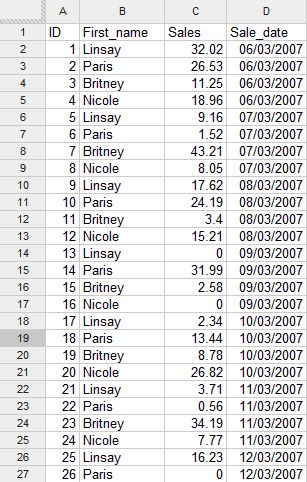
our data set like this
s
-
try this formula
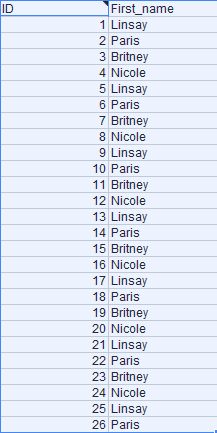
=QUERY(A:D;”select A,B”;1) the result will be as show in the below image
-
We have some special keywords called functions, Functions are bits of code that perform an operation on a value or values. The first we will see is to perform a mathematical operation on a column. We will see Sum function which by totaling the values in a column designated by parentheses.
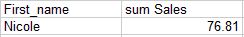
suppose we want to Sum Column C where the Column B is Nicole
=QUERY(A:D;”select B, Sum(C) where B = ‘Nicole’ group by B”;1)
-
the result will be
-
Note:
(1) you have to use S capital in the Sum followed by column you want sum in parentheses
(2) whenever you are using the group by clause same column has to be selected in the select clause otherwise you may get value error
(3) condition you want the check in the column B has to be in single quote
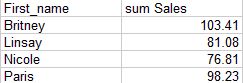
this can be sorted using the order by clause
=QUERY(A:D;”select B, Sum(C) where B <>” group by B order by B asc”;1)
the result will be
Note:
(1) observe the column 1 has been sorted in ascending order
(2) to get the the descending order you can use the desc instead of asc
-
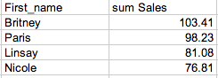
you can also sort the based on the result of the Sum(C)
=QUERY(A:D;”select B, Sum(C) where B <>” group by B order by Sum(C) desc”;1)
the results will be
Note:
(1) we have sorted data by descending order based on Sum of sales
(2) you have to follow the order of clause listed above
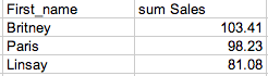
We can also limit the results top 3 or top 2 using the limit clause
=QUERY(A:D;”select B, Sum(C) where B <>” group by B order by Sum(C) desc limit 3″;1)
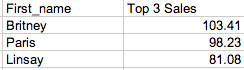
We can also the name the column sum Sales as Top 3 sales
=QUERY(A:D;”select B, Sum(C) where B <>” group by B order by Sum(C) desc limit 3 label Sum(C) ‘Top 3 Sales'”;1)
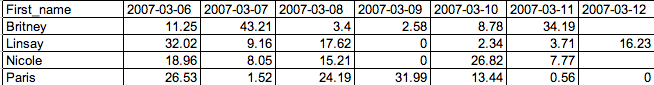
We can also pivot the data based on date in the D column.
=QUERY(A:D;”select B, Sum(C) where B <>” group by B pivot D”;1)
Note:
(1) You might have observed the column D is not selected the select clause
(2) Date are formatted in yyyy-mm-dd format
(3) pivot is unique to google Sheets Query function
-
In the next blog post we will see how to manipulate data using the cell value
- the link the spreadsheet is as follows:
- https://docs.google.com/spreadsheets/d/12B3C3NPLcZ1Dpa0jNvF2ClPWvLJBznCdHif6–m334c/edit?usp=sharing

Pingback: Single column manipulation using query function | anandexcels
Thank you.
Col1, Col2 – that is what I am looking for.
Hello, this is really helpful in trying to understand how to use the query function. In your example above =QUERY(A:D;”select B, Sum(C) where B ” group by B order by Sum(C) desc”;1) can you please explain the meaning and purpose of “where B “?. Many thanks
Dear Andrew,
where B” is used to eliminate the blank rows from the data set since i have used the A:D ( it is and open range). If you use A1:D10 you do not require the Where B”
the advantage of open range is if you add data the function continue to work with additional data
Thanks. That’s helpful. For some reason the (less than followed by greater than) symbols I included above have not come through onto the page.
Pingback: Quick Tips to Format Data to Make your Data Sets Flexible | Content Generator
Pingback: Quick Tips to Format Data to Make your Data Sets Flexible
Hi! Thanks for explaining this function so well! I am using query and importrange to draw certain data from a different spreadsheet. I would then like to add some more columns of data which will be written manually into the new sheet. The problem occurs if a row is then added or deleted in the source spreadsheet. I need my manually entered data to move along with the corresponding imported data. Do you have any idea if this is possible? I’ve searched everywhere but can’t figure it out. Thanks!
Try using Arrayformula. Like this: =ARRAYFORMULA(IFERROR(….your formula here…,””)). Arrayformula takes in array arguments and extends formulas for as many rows as the array argument has. So you can include an entire column (i.e. A:A or B5:B) as an argument to have it cover every possible row in the sheet.
This is why I love Google Docs more than Excel. It has so much more potential in my opinion. But it lacks the firepower.
Pingback: Quick Tips to Format Data to Make your Data Sets Flexible « Universalplusjl's Blog
Whenever I do =QUERY(A:D;”select B, Sum(C) where B = ‘Nicole’ group by B”;1), I always get a pre-formatted fields with sumSales, is there a way to remove that formatting and just get the sum of those cells?
Thanks!
you can use Label such as this
=QUERY(A:D;”select B, Sum(C) where B = ‘Nicole’ group by B Label Sum(C) ‘Total’”;1)
Dear Alex
try this formula
=QUERY(A:D;”select B, Sum(C) where B = ‘Nicole’ group by B Label Sum(C) ‘Total’,B ‘Category’ ”;1)
Hi! Thanks so much for this post!!
I am trying to pass some data from one sheet to another, only if the product has been marked as sold = 1.
The formula I am using is: =QUERY(Sheet1!A:C;”select A, B, C where C=1”;1) but I get an error and don’t know how to correct it.
Please help 🙂
Link to the spreadsheet: https://docs.google.com/spreadsheets/d/1DLqSee84FxLB1tndu36X90QowKFQUlgA7JzGMwbU1j8/edit?usp=sharing
Thank you!!!!
Dear Sara
the formula working as expected
=QUERY(A:C,”Select * where C=1″,1)
have a look at the following link
https://docs.google.com/spreadsheets/d/1ghB_STHm8yD45Jh0pVBgCgcavzprzmDPIVD6NEaGyIo/edit?usp=sharing
Hi, Is there the equivalent of the SQL “IN” clause? eg select Col1, Col2 where Col3 in (“eggs”,”bacon”, “toast”,”corn-flakes”).
To be honest I haven’t see any mention of it, but thought it was worth asking.
Reblogged this on Power to Build.
I am trying to pull data from a different tab within the same work book; the purpose is to update a list as new products are added based on product category.
Hi,
I made a simple query function as this: =QUERY(range,”select *”,1), in my Google Spreadsheet, but it dose not show any letters, it shows only fields that contains numbers.
Can you assist me with this ?
Thank you.
I am actually delighted too read his web site posts which includes plenty of helpful
facts, thanks for providing such information.
Hello, can i make duplication of query table as i did in microsoft excel with power query > for sample, in tab1 i have main table then tab2, tab3, tab4 is automatically update table from tab1. That means I want to insert data only in tab1 then I can continue to add more columns in tab2 and tab3.
Many thanks
how i do add in =QUERY(A:D,”select B, Sum(C) where B ” group by B order by Sum(C) desc”,1) one more filter e.g and D > ’06/03/2007′ and D < '10/03/2007'
This does not work:
=QUERY(A:D,"select B, Sum(C) where B ” and D > ’06/03/2007′ and D < '10/03/2007' group by B order by Sum(C) desc",1)
is it possible to make the “where” condition variable picking value from a cell?
Example:
=query(Sheet1!A1:C10; “select * where A = [value in D1]”; 1)
replace this [value in D1] with ‘”&D1&”‘
Thanks!
We’re a grooup off volunteers and opening a new scheme in our community.
Your web site offered us with valuable injfo too work
on. You have done a formidable job and our whol community
will bbe grateful to you.
Hi Anand
This is super-helpful. How can I use limit to deliver not the top n results (eg limit 3) but results p to q from the list?
This is super-helpful.