VLOOKUP

Vlookup is one of the most powerful functions in Spread sheets. So many people use Vlookup as a daily function, and is most useful in searching a table, looking for the same names, field or identifier and then spitting out an output based on that search criteria. It may sound difficult, but is quite easy

The VLOOKUP function retrieves an item from a table and returns it to a cell or formula.

The Syntax of the function is

VLOOKUP(search_criterion, array, index, sort_order)

The VLOOKUP:

1) Looks for a value in the leftmost column of a table

2) And then returns a value in the same row from a column you specify

3) By default, the table must be sorted in an ascending order

The VLOOKUP function has four arguments:

1) search_criterion: This is the items that the VLOOKUP looks at before it goes over to the table and looks it up. Once the VLOOKUP goes over to the table, it looks in the leftmost column to try and fine the value

2) array : is the table (database) that you are looking a value up in

3) index : is the number of the column that has the value you want to get and return back to the cell (the leftmost column of the table is considered 1). For this argument you can use the COLUMNS or ROWS functions to increment numbers.

4) sort_order : is a 0 when you are looking up an exact value (like a word) and 1 or omitted when you are looking up an approximate value (like in tax tables where you want to find the row that is equal to the lookup_value or greater than, but less than the next value in the leftmost column.

Notes:

• If index is less than 1, the VLookup function will return #VALUE!.
• If index is greater than the number of columns in table_array, the VLookup function will return #REF!.
• If you enter FALSE for the not_exact_match parameter and no exact match is found, then the VLookup function will return #N/A.

(1) The search_criterion argument is the “number that we are looking up.”.

• NOT case sensitive (TOM=tom=ToM=tOM)
• Cannot be longer than 255 characters.
• Can be a number, text, logical value, or a name or reference that refers to a one of these

(2) The array argument is the lookup table and can contain one or more columns.

• The first column is the lookup column
• The column with the values to return can be in any of the columns(1,2,3, and so on)
• If you are doing an approximate match, the first column must be sorted smallest to biggest.
• If you are doing an exact match, the first column does not need to be sorted.

(3) The Index argument is a number (1,2,3, and so on) that represented the column in the table_array that has the value to return to the cell.

(4) The sort_order argument tells the VLOOKUP function whether you are doing an approximate match or an exact match or an exact match when looking up a value.

If you are doing an approximate match, the first column must be sorted smallest to biggest(ascending)

If there are duplicates in the first column, VLOOKUP will choose the first one listed.

Now let see and understand the working of VLOOKUP function:

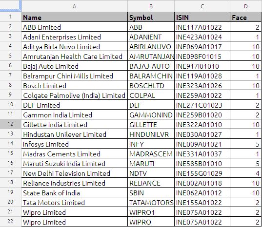
The sample data is taken from NSE (National Stock Exchange) of India web site, the first column is name of the company, second column in NSE stock symbol, third column is ISIN number and the  fourth column is face value of stock script.

the data used in this example available at the end of the post

suppose we want stock symbol of Gillette India Limited in cell B5 the formula will be

= VLOOKUP(A24,A2:D21,2,FALSE)

 in the above example search_criterion argument is A24 it is name of the stock we want to search in the data base or table.

array argument is table array which is from A2 to D21

index argument is the column index number in the above example it is  2 which stock symbol corresponding to script.

sort_order in the above example sort_order is FALSE because we want to exact match.

If there is no match for the search_criterion, the VLOOKUP spit the data one row above the nearest value.

In the above example the APPLE COMPUTERS INC does not have any value in the table, but since we have put the Sort_order as TRUE which is nothing but approximate match. we have got the AMRUTANJAN.

In case of duplicate values the VLOOKUP function return the value in the first place.

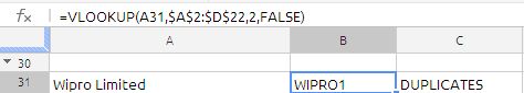
in the data table if you see A21 and A22 has the same value, VLOOKUP function will return first value only. this is big constrain in the  VLOOKUP function.

the formula in cell B33 is

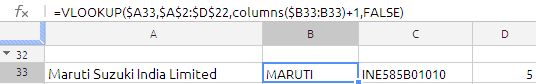
=VLOOKUP($A33,$A$2:$D$22,COLUMNS($B33:B33)+1,FALSE

If we drag it across we will get the data from  Symbol,ISIN, Face. the only logic inside the formula is correct use of relative reference and use of COLUMNS function which is column increment in the  above formula

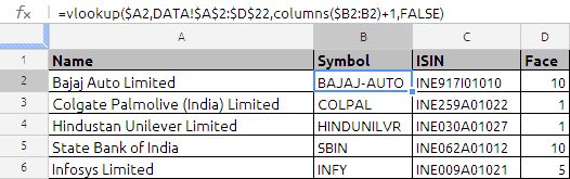
in the above example the formula used in cell B2 is =VLOOKUP($A2,DATA!$A$2:$D$22,COLUMNS($B2:B2)+1,FALSE) drag it down and   cross

the above formula will fill the column B, C & D.

the above formula is traditional way of writing. But same can be modified in the google docs array formula as shown in the below example:

this is single most efficient, no dragging is required.

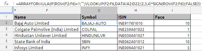
the formula used in cell G2 is =ARRAYFORMULA(IF(ROW(F2:F6)=1;””;VLOOKUP(F2:F6,DATA!A2:D22;{2,3,4}*SIGN(ROW(F2:F6));FALSE)))

most noticeable point is use of {2,3,4} which is array of column numbers which we want to extract. SIGN function is used to convert the true /false to 1 and 0

VLOOKUP is more versatile, most used function, i am only trying to explain with basic futures only.

.

You can download the workbook at the following link

https://docs.google.com/spreadsheet/ccc?key=0AjeH8BMrOPivdGRZZXJvUXpFTTRIb290SExDYm5pWHc